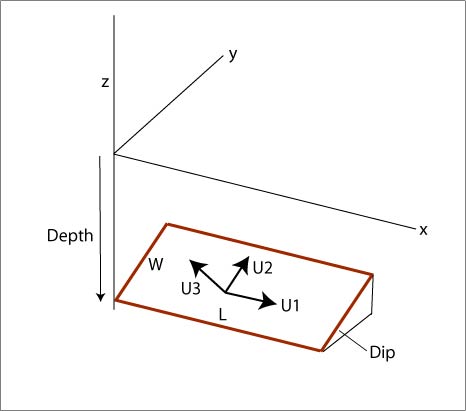
Fig. 1 Indexing of nodes on the fault surface.
Last manual update: July 24, 2023.
Warning: This version is still in progress, not everything works as described in the manual. Do NOT redistribute the program.
TDEFNODE is a Fortran program to model elastic lithospheric block rotations and internal strains, locking on block-bounding faults, and transient sources such as earthquakes, afterslip, slow-slip, volcanic sources, etc. Block motions are specified by spherical Earth angular velocities (Euler rotation poles) and interseismic backslip is applied along faults that separate blocks, based on the routines of Okada (1985; 1992). The faults are specified by lon-lat-depth coordinates of nodes (forming an irregular grid of points) along the fault planes. The parameters are estimated by simulated annealing or grid search.
This version differs from DEFNODE largely in that time dependent deformation and data can be considered. GPS time series and multiple InSAR interferograms can be modeled using the steady block model, as in DEFNODE, with the addition of time-dependent sources. This version also allows the blocks to be built from the fault segments (+mkb flag).
DISCLAIMER I make no guarantees whatsoever that this program will do what you want it to do or what you think it is doing. It has more than 30,000 lines of code and I guarantee some bugs are there. I have not tested every option thoroughly and have not documented every option. However, I use it extensively for my own research as is. I am happy to hear about tests you perform and will try to fix any bugs you discover.
REQUEST Please do not make changes to the code and/or re-disribute it. I am happy to help with any improvements or changes.
The program can solve for:
Data to constrain the models include:
Prior users: The program is greatly modified from earlier versions. Many commands are the same, but many are also changed, and there are many new ones. It is advised to browse the commands to see the changes.
INSTALLATION: Before compiling, do the following:
See README
ABBREVIATIONS used:
NOTES:
Directories: All output will be put into a directory specified by the MO: (model) command. The program also produces a directory called 'gfs' (or a 3-character, user-assigned directory name) to store the Green's function files.
Poles (angular velocities) and blocks: You can specify many poles and many blocks (dimensioned with MAX_poles, MAX_blocks). There is NOT a one-one correspondence between poles and blocks. More than one block can be assigned the same pole (ie, the blocks rotate together) but each block can be assigned only one pole. Poles can be specified as (lat,lon,omega) or by their Cartesian components (Wx, Wy, Wz). Poles can be fixed or adjusted. Angular velocities are relative to the center of the Earth and obey the right-hand rule. Looking from above (in map view), negative rotations will be clockwise.
Strain rates and blocks: The uniform, horizontal strain rate tensors (SRT) for the blocks are input in a similar way as the rotation poles. Each SRT is assigned an index (integer) and blocks are assigned a SRT index. As with poles, more than one block can be assigned to a single SRT. Velocities are estimated from the SRT using the block's centroid as origin (default) or a user-assigned origin (see ST:); if multiple blocks use the same SRT assign an origin for this SRT (with ST: option). SRTs can be fixed or adjusted.
Faults and blocks: Faults along which backslip is applied are specified and must coincide point-for-point at the surface with block boundary polygons. However, not all sections of block boundaries have to be specified as a fault. If the boundary is not specified as a fault it is treated as free-slipping and will not produce any elastic strain (ie, there will be a step in velocity across the boundary). By specifying no faults, you can solve for the block rotations alone.
Making blocks from faults: The program can now make the blocks from the faults alone using the algorithm of W. R. Franklin. This is done with the +mkb flag. However, the faults input, when connected, must together form a series of closed polygons. In other words, every point (surface node) must be on at least 2 fault segments. If they don't, an error 'Fix unmatched segment' is produced and the program stops. The unmatched segments are written to the screen and you must fix them. To close blocks, 'pseudo-faults' can be used - they are 'faults' with nodes only at the surface and are treated as free-slip boundaries (see FA:). With this option, you do not need to input blocks (BL:) separately but do need to assign block names with the BC: option.
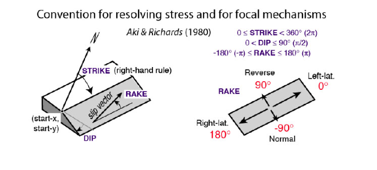
Fault nodes: Fault surfaces are specified in 3 dimensions by nodes whose positions are given by their longitude and latitude (in degrees) and depth (in km, positive down). Nodes are placed along depth contours of the faults and each depth contour must have the same number of nodes. Nodes thus form an irregular grid on the fault surface. Nodes are numbered in order first along strike, then down dip. The figure below shows the numbering system for the nodes. Strike is the direction faced if the fault dips off to your right. Faults cannot be exactly vertical (90o dip) as the hangingwall and footwall blocks must be defined. The fault geometry at depth can be built either by specifying all the node coordinates individually or automatically using the DD: and ZD: options.
The coupling fractions (ratio of locked to total slip, called phi) or slip amplitude (for coseismic applications) are either specified or estimated at the nodes. The 'slip deficit rate vector' is phi is multiplied by the slip vector V at the node, where V is estimated from the angular velocities. The slip rate deficit gives rise to the elastic deformation around the fault. For coseismic, phi is the fault slip amplitude and the unit vector V gives the slip direction.
The elastic deformation is calculated by integrating over small patches (quadrilaterals) in the regions between the nodes (see figure above). The Okada method is used to calculate surface velocities while applying backslip at a rate of -V Phi (or V Phi for coseismic) on each of these little patches. Because the Okada formulas used are for rectangular patches, the sizes of the interpolated patches should be kept small (less than a few kilometers). As the patches get smaller their deviations from rectangles matters less (the point source approximation).
The distribution of interseismic locking or co-seismic slip on the fault can be parameterized in several ways (see FT: option for details). The nodes can be treated as independent parameters or can be grouped such that multiple nodes have the same phi value. The distribution of slip can also be set to one of a few specified functions of depth (exponential, boxcar, or Gaussian) along depth profiles, called z-profiles. In this case, the parameters for the function can be varied along strike on the z-profiles. This version allows 2D Gaussian distributions of slip on the fault surface that may be suitable for earthquakes or slow slip events.
Transients: are represented by combining a spatial slip distribution with a temporal slip distribution. Use the ES:, EI:, EX: and EF: commands and optionally ER: and ET:. Some other commands are applied to transients by putting a 't' in the third column. For example SMt: applies smoothing to transient slip distributions.
Green's functions: If you are performing an inversion, the program uses unit response (Green's) functions (GFs) for the elastic deformation part of the problem since the inversion method (downhill simplex) has to calculate numerous forward models. The GFs are put in a directory called 'gfs' (or a user-specified directory using GD: option) and the files are named with the form gf001001001g, gf001002001g, etc. First 3 digits are fault number, next 3 are the along strike (X) node index, the next 3 are the downdip (Z) node index, the final letter is the data type; g - GPS, i - InSAR, t - Tilts, s - strain rates. Once you have calculated GFs for a particular set of faults you can use these in inversions without recalculating them (see option GD: ). The GFs are based on the node geometry, GPS data, InSAR data, strain tensor data, and tilt rate data so if you change the node positions or ADD data, you need to re-calculate GFs. If you REMOVE data, you do not need to recalculate GFs. You can add or subtract slip azimuths, slip rate, and rotation rate data without re-calculating GFs since those data are calculated from the rotation poles only. If you change a node position the program will detect the change it and re-calculate only the necessary GFs.
If you add GPS vectors, the program will detect that their GFs may be missing but will not automatically calculate them. In this case, re-calculate all the GFs.
The GFs are the responses at the surface observation points to a unit velocity (or displacement) in the North and East directions at the central node. The slip velocity is tapered to zero at all adjacent nodes.
Data files and weighting: Data files are generally in free-format but the information must be in the correct order as outlined below. Multiple data files can be specified and they are all read in and used. An uncertainty scaling factor F can be applied to each data file; this number is multiplied by the data standard errors given in the file. Since the weight applied is the inverse of the datum variance, the weight of the datum will be multiplied by F-2. If s is the standard deviation of the datum given in the file, the new standard deviation s' = sF and the weight =s' -2 = (sF)-2. Data covariance is used when the correlation coefficient is given for GPS vectors.
Some data types can be entered within the control file itself.
Inversion: The inversion finds the set of parameters that minimizes the sum of the reduced chi-squared statistic Xn2 plus any penalties:
Xn2 = [ SUM r2/(sF)2] /dof
where r is the residual, s is the standard deviation, F is the scaling factor just described, and dof is the degrees of freedom (number of observations minus number of free parameters). The SUM is over all data. For angular data, the r/s is determined using the equation of DeMets et al. (1990).
Penalties are used to keep parameters within specified bounds and to apply smoothing of slip distributions.
Minimization of Xn2 + Penalties is performed by the simulated annealing technique (see Press et al. 1989), grid search or linear inverse. These are controlled by the SA: (simulated annealing), GS: (grid search), and IC: (iteration control) commands.
Units:
Coordinates:
Miscellaneous notes and suggestions:
ITERATING: The IC: option controls the iterations; 1 for simulated annealing, 2 for grid search, 3 for linear inversion. While iterating, press 'q' to stop or 's' to go to the next step in the IC: list. During grid search press 'n' to jump to the next step of the grid search. Linear inversions can be used only for the simplest, linear problems like solving for poles and strains without fault locking.
Screen output during simulated annealing:

 It      Ptot   D_Chi      Penalty  Parameters -->

It         iteration number
Ptot       total penalty
D_Chi      data reduced chi**2
P_sum      sum of all penalties
Parameters parameter values


Screen output during gradient grid search:

  No Type   Ptot   D_Chi       P_sum  Parameter    Change Max_P Steps

No         parameter number
Type       parameter type code
Ptot       total penalty
D_Chi      data reduced chi**2
P_sum      sum of all penalties
Parameter  parameter value
Change     change in parameter value
Max_P      source of maximum penalty (see Penalty codes)
Steps      number of steps grid search made
Parameter types
Parameters are identified by a number and a 2-letter code.
Interseismic parameter types
  1 vp - GPS velocity field pole component (deg/Ma)
  2 bp - block pole component (deg/Ma)
  3 sr - strain rate component (nanostrain/yr)
  4 ph - coupling factor phi (unitless)
  5 wg - Wang gamma value (unitless)
  6 z1 - minumim locking depth; Wang or Boxcar (km)
  7 z2 - maximum locking depth; Wang or Boxcar (km)
  8 mi - interseismic mean locking depth for Gaussian phi(z) (km)
  9 ms - interseismic sigma of locking depth for Gaussian phi(z) (km)
 10 vb - velocity bias for a field, East, North or Up (in mm/yr)

Transient parameter types
 21 ln - Longitude of source (deg E)
 22 lt - Latitude of source (deg N)
 23 zh - Depth of source (km below surface)
 24 d1 - W-width [plane] or W-Sigma [2D Gaussian] (km)
 25 am - Amplitude (mm or mm/yr)
 26 d2 - X-width [plane] or X-Sigma [2D Gaussian] (km)
 27 to - Transient origin time (decimal year)
 28 tc - Transient time constant [Gaussian width, boxcar duration, decay constant] (days)
 29 mr - Transient migration rate (km/day)
 30 ma - Transient migration azimuth (degrees)
 31 st - Strike of fault plane (deg)
 32 dp - Dip of fault plane (deg)
 33 rk - Rake on fault plane or azimuth of slip (deg)
 34 az - Azimuth of X-axis for 2D Gaussian (deg)
 35 rd - Polygon radius (km)
 36 ta - Amplitude of stf element for transient (mm/yr)
 37 ga - 1D Gaussian amplitude (mm/yr)
 38 gm - 1D Gaussian mean depth (km)
 39 gs - 1D Gaussian spread (km)
 40 ba - 1D Boxcar amplitude (mm/yr)
 41 b1 - 1D Boxcar minimum depth (km)
 42 b2 - 1D Boxcar maximum depth (km)
 50 mo - Moment (Nm)
Some parameters do not appear on this list. They are estimated by regression at each iteration. These include: GPS time series offsets (and slopes if estimated); GPS time series seasonal amplitudes; and InSAR planar and troposphere offset parameters
Penalty codes: Parameter values can be limited globally by using the PM: option or individually for transients with the EX: option. When the parameter goes outside this limit, a penalty is applied. The penalties have the following codes:
Code Parameter
 1 - GPS velocity field rotation pole component (deg/Ma)
 2 - block pole component (deg/Ma)
 3 - strain rate component (nanostrain/yr)
 4 - coupling factor phi (unitless)
 5 - Wang gamma value (unitless)
 6 - minumim locking depth; Wang or Boxcar (km)
 7 - maximum locking depth; Wang or Boxcar (km)
 8 - interseismic mean locking depth for Gaussian phi(z) (km)
 9 - interseismic sigma of locking depth for Gaussian phi(z) (km)
80 - damp phi amplitudes
81 - damp phi gradient
82 - damp phi spread
83 - damp phi Laplacian
89 - damp block strain rates (flag +dst)
94 - downdip decrease in phi
95 - bounds on moment rate
96 - hard constraints
97 - max depth > min depth (parameter types 6 and 7)

For transients:
EEPP - transient constraints (EE=event number, PP = transient parameter number)
       (eg 0521 is longitude for event 5)
EE21 ln - Longitude of source (deg E)
EE22 lt - Latitude of source (deg N)
EE23 zh - Depth of source (km below surface)
EE24 d1 - W-width [plane] or W-Sigma [2D Gaussian] (km)
EE25 am - Amplitude (mm or mm/yr)
EE26 d2 - X-width [plane] or X-Sigma [2D Gaussian] (km)
EE27 to - Transient origin time (decimal year)
EE28 tc - Transient time constant [Gaussian width, boxcar duration, decay constant] (days)
EE29 mr - Transient migration rate (km/day)
EE30 ma - Transient migration azimuth (degrees)
EE31 st - Strike of fault plane (deg)
EE32 dp - Dip of fault plane (deg)
EE33 rk - Rake on fault plane or azimuth of slip (deg)
EE34 az - Azimuth of X-axis for 2D Gaussian (deg)
EE35 rd - Polygon radius (km)
EE36 ta - Amplitude of stf element for transient (mm/yr)
EE37 ga - 1D Gaussian amplitude (mm/yr)
EE38 gm - 1D Gaussian mean depth (km)
EE39 gs - 1D Gaussian spread (km)
EE40 ba - 1D Boxcar amplitude (mm/yr)
EE41 b1 - 1D Boxcar minimum depth (km)
EE42 b2 - 1D Boxcar maximum depth (km)
EE50    - moment of event
EE51    - planar source extends above surface
EE54    - damp tau values or tau smoothing
EE55    - polygon
EE56    - source on fault
EE60    - damp slip amplitudes
EE61    - damp slip gradient
EE62    - damp slip spread
EE63    - damp slip LaPlacian
EE97    - max depth > min depth (parameter types 41 and 42)
CONTROL FILE
The program reads the model and all controls from an ASCII file. Some data can be in the control file. The control file format is described here.
Lines in the control file comprise a keyword section and a data section. The keyword section starts with a 2-character
keyword (they have to be in the first 2 columns) and ends with a colon (:). Normally only the first 2 characters of the keyword are used
so in general any characters between the 3rd
character and the : are ignored. The third character is sometimes used to specify a format or a transient input as outlined below.
THE KEYWORD MUST START IN THE FIRST COLUMN OR THE LINE IS IGNORED.
Case does not matter. Comments may be added after a second colon in the line.
The data section of the input line goes from the colon to the end of the line (or to a second colon) and its contents depend on the keyword. In a few cases the data section comprises multiple lines (always BL:, FA:, and PV:, and sometimes NN: and NV:).
For example, the key characters for a fault are 'FA' and this has two arguments, the fault name and the fault number, so the following lines are correct:
fa: JavaTrench 1
fault: JT 1
fault (Java trench): JavaTr 1
FA: JT 1  : this is the Java Trench
but
thrust fault: 1
 fault: JT 1
fault 1 : JavaTrench
are not valid.
Some notes on input lines:
Multiple instances can exist in the control file for somew types of input; the program uses the last valid occurrence it finds. For example, if the following pole specification lines are in the control file
pole: 1 -20 40 .2
pole: 1 -19 33 .1
the values (-19, 33, .1) will be assigned to pole 1, over-writing the earlier instance.
An exception to this rule pertains to data files, that are all used.
The order of the statements in the control file should not matter since the program reads it multiple times. The control file can contain lines after the end of input (EN:) statement and these are ignored.
The control file can contain multiple models through the use of the MO: - EM: structure.
COMMANDS
(++ new to TDEFNODE; ** not for general use or in development; -- not used any more)
Descriptions of Key Characters and input format:
Key characters and formats. Examples are given at bottom. Optional third-character control entries are shown in boxed brackets [ ]. Squiggly brackets { } show other optional inputs. MODL = 4-char model name.
AV: X1 Y1 X2 Y2 X3 Y3
Add (X3,Y3) to boundary between (X1,Y1) and (X2,Y2)
if X3=0 and Y3=0 place new point halfway between (X1,Y1) and (X2,Y2)
av: 236.0 39.0 238.0 39.0 237.0 39.0
BC: NAME X Y M N
NAME = 4-character name of block
X = longitude of point within block (near center)
Y = latitude of point within block (near center)
M = Rotation pole index for block
N = Strain rate tensor index for block
This command is needed for each block if they are being built from the faults (+mkb flag is set).
bc: NoAm 263.0 42.0 1 0
bc: JdFa 222.0 42.0 2 0
bc: EOre 230.0 43.0 3 1
BL: NAME  M  N {optional filename}
 followed by a multiline data section
Not needed if blocks are built from faults.
NAME = 4-character name of block
M = Rotation pole index for block (overridden by BP: option)
N = Strain rate tensor index for block (overridden by BP: option)
filename = optional file containing block outline
Multiline data section (alternatively, contents of filename)
First line: Number of corners outlining block, { CentroidX CentroidY }
CentroidX = x coordinate of block centroid (optional)
CentroidY = y coordinate of block centroid (optional)
For each corner, one coordinate pair (lon, lat) in each line
bl: NOAM 1 1
4 50 50
-135  55
-130  44
-100  44
 260  55

 or

bl: NOAM 1 1 NOAM.block

where NOAM.block is a file contining:

4 50 50
-135  55
-130  44
-100  44
 260  55
bl: NOAM 1 1
9999 50 50
-135  55
-130  44
-100  44
 260  55
 9999 9999
BP: NAME N M
Block NAME uses pole of rotation N and strain rate tensor M. This overrides the assignments given in BL: or BC: option. Set to 0 if no pole or strain tensor is used.
bp: NoAm 1 0
bp: JdFa 2 0
bp: EOre 3 1
BR: Bnew BLK1 BLK2 ...
Rename one or more blocks with a new name Bnew. The new name is applied to any block names, input data or faults that refer to the old blocks. For example:
BR: Blk3 Blk1 Blk2 Blk4will replace any instances of Blk1, Blk2, or Blk4 with Blk3. If you combine 2 or more blocks and want to keep an existing name, put that block name first. For example, say there are 2 independent blocks NoAm and Rcky, that you want to combine and make any data that refers to Rcky now refer to NoAm, use:
br: NoAm Rcky
CF: F1 F2Connect 2 faults at their intersection. Where fault #F1 and fault #F2 intersect at the surface, force deeper nodes to also intersect by moving nodes (at same depth) from both faults to the average position of the two nodes. Both faults must have their nodes at the same depths for this to work.
cf: 5 7
Remove data/controls read in thus far.
cl: gps svsUp to 8 per line. Multiple lines allowed.
CO:Continue reading data from file (turns off SK: skip mode).
DR: min_lon max_lon min_lat max_lat {min_time max_time}
DR: 220.0 250.0 32.0 45.0 2004.0 2012.5
Time window is optional. The default 'max_time' is the date of the current run. It is sometimes used to give the duration of transients that are still ongoing.
DSx: Name filename N F Smin Smax NU T1 T2 E N U
The third character specifies the input format:
  x   Format
      Lon  Lat  De Se Dn Sn Dz Sz Site T1 T2 (default; x= nothing)
  1   Lon  Lat  De Dn Dz Se Sn Sz Site T1 T2
  2   Lon  Lat  De Dn Se Sn Site Dz Sz T1 T2
  3   Lon  Lat  De Dn Se Sn rho Site T1 T2   (horizontal only; psvelo format)
  4   Lon  Lat  Dz Sz Site T1 T2             (vertical only)
  5   Lon  Lat  De Dn Se Sn Site T1 T2       (horizontal only)
where:
Lon = longitude
Lat = latitude
De = East displacement, mm
Dn = North displacement, mm
Dz = Vertical displacement, mm
Se = East sigma, mm
Sn = North sigma, mm
Sz = Vertical sigma, mm
rho = EN correlation
T1 = start of time over which displacement is measured (overrides DS: entry)
T2 = end of time over which displacement is measured (overrides DS: entry)
Site = site name
ds2: DIS1 quake.dat 3 1.0 0.2 0.0 0.0 2007.12 2007.23 1 1 0
DV: X1 Y1
Delete all (X1,Y1)
Warning: Deleting endpoints of the block/fault segments will cause a problem when building blocks from faults. Be sure you know what you are doing.
dv: 236.2 -14.1
DW: I F T1 T2 { N N ... }
Write to files the displacements at nodes and slip distribution for fault number F for transients between times T1 and T2 (in decimal years).
Transients to be summed can be listed or the default is to use all transients on the fault F.
Output file names are MMMM_time_III.nod are MMMM_time_III.atr where I is the index given.
dw: 1 1 2008.3 2008.6 1 2 3
EC: Shear_modulus Lambda Poisson_ratio
ec: 4.0e10 4.0e10 0.25
EF: N P1 P2 P3 ...For transient source N, adjust parameters listed.
ef: 2 ln lt zh st dp rk am
See parameter codes in ES:.
If the code is 'cl' this clears the free parameters for this event (fixes them).
ef: 999 clfixes the free parameters for all events.
EI: N N NUse transient sources listed by N.
ei: 1 2 3
EM:End of model input section (no arguments).
EN:End of control file (no arguments), anything in the file after this line is ignored.
EQ: F1 X1 Z1 F2 X2 Z2Make two nodes on different faults have same value of phi in the inversion. F, X, and Z are the indices for the nodes. Applies to fault types FT: 0 and 1 only.
EQp: F1 X1 Z1 F2 X2 Z2Set node position to one from other fault, second node listed takes position of first
EQt: T1 T2 P1Equate two transients parameters. T1 and T2 are transient numbers, P1 is the parameter number (see ES:)
EQt: T1 X1 Z1 T2 X2 Z2Equate slip of two transients at a nodes. [**** Not working ****]
eq: 1 4 2 2 1 2forces the node of the first fault which is fourth along strike and second downdip to have the same phi as the second fault's first node along strike and second downdip.
ER: I N Damp R1 R2 R3 ... Rn
er: 2 6 0.0 30.0 40.0 50.0 40.0 30.0 30.0
To adjust radii, put 'rd' in EF: option.
ES: I list parameter codes and valuesI = source number
See also EX: for parameter constraints, and EF: to adjust parameters.
Parameter codes: No Code Parameter (units) 21 'ln' longitude (deg) 22 'lt' latitude (deg) 23 'zh' depth (km) 24 'd1' down-dip width (km), semimajor axis for Spheroid 25 'am' slip rate amplitude (mm/yr) 26 'd2' along-strike width (km), A/B for Spheroid 27 'to' origin time (years) 28 'tc' time constant (days) 29 'xr' East or strike migration rate (km/day) 30 'wr' North or dip migration rate (km/day) 31 'st' strike azimuth (deg) 32 'dp' dip angle (deg) 33 'rk' rake or slip azimuth (deg) 34 'az' azimuth of Gaussian X-width (deg) 35 'rd' polygon radii (km) 36 'ta' tau amplitude (mm/yr) 37 'ga' 1D Gaussian amplitude (mm/yr) 38 'gm' 1D Gaussian mean depth (km) 39 'gs' 1D Gaussian sigma (km) 37 'ba' 1D Boxcar amplitude (mm/yr) 38 'b1' 1D Boxcar mean depth (km) 39 'b2' 1D Boxcar sigma (km) Other codes: 'fa' fault number 'sp' Spatial source type (0 to 11; see below) 'ts' Time dependence type (0 to 6; see below) 'sa' slip azimuth control (0 or 1; see below) 'mt' slip migration type (0 for bi-lateral; 1 for circular) 'mo' moment Spatial source type (sp)Migration: The source can migrate spatially across the Earth's surface or across the fault (via +ndl flag). The delays are based on an elliptical front due to different along strike and down-dip migration rates. The source starts at a time To (to; Parameter 27) at a Longitude (ln; Parm 21) and Latitude (lt; Parm 22). The source migrates along strike (xr; Parm 29) and down-dip (wr; Parm 30). If +ndl flag is set the migration is along the surface of the fault; if -ndl flag is set the source migrates relative to the surface (an apparent migration rate as recorded by the sites). The former is more exact but runs slower.
1 Independent nodes (use smoothing)
2 not used 3 1D Boxcar S(z) S(z) = 0 (z < Z1); = A (Z1 <= z <= Z2); = 0 (z > Z2) Parameters: ba = Amplitude of boxcar; b1 = upper depth; b2 = lower depth
4 1D Gaussian S(z) S(z) = A * Ga * exp{-0.5*[(z-Gm)/Gs]**2} (see PNt: also) Parameters: ga = Amplitude; gm = mean depth; gs = depth spread
5 not used 6 Gaussian 2D slip source S(x,w) = A * exp[-0.5*(dw/d1)**2] * exp[-0.5*(dx/d2)**2] x - along strike axis; w - down dip axis dx, dw = distance from node to center of slip (Lon, Lat) Parameters: Am = Amplitude; d1 = down-dip length; d2 = along-strike length
7 Boxcar 2D slip source S(x,w) = A (if |dx| < d2 and |dw| < d1 ); = 0 otherwise x - along strike axis; w - down dip axis dx, dw = distance from node to center of slip (Lon, Lat) Parameters: Am = Amplitude; d1 = down-dip length; d2 = along-strike length
8 Polygon, uniform slip source (needs ER: line) S(x,w) = A (if node within polygon); = 0 otherwise
9 Earthquake slip source (double couple not on block bounding fault; Okada U1 and U2) Parameters: Am = Slip; st = strike; dp = dip; rk = rake; zh = depth; ln = longitude; lt = latitude; d1 = down-dip length; d2 = along-strike length
10 Mogi source (Segall 2010 eqn 7.14) Parameters: am = amplitude in millions of cubic meters (Mm3) volume change; ln = longitude; lt = latitude; zh = depth
11 Planar expansion source (not on fault; Okada U3) Parameters: Am = Slip; st = strike; dp = dip; zh = depth; ln = longitude; lt = latitude; d1 = down-dip length; d2 = along-strike length
12 Prolate spheroid (Yang et al.) Parameters: ln = longitude; lt = latitude; zh = depth; am = expansion rate; st = strike; dp = dip; d1 = semi-major axis length (km); d2 = ratio of semi-major to semi-minor lengths (a/b)
Time dependence type (ts) S(t) is slip velocity; D(t) is displacement; A is amplitude; To is origin time (decimal years), Tc is a time constant (days)
0 impulse (default) S(t) = 0 (t < To and t > To); S(t) = A (t = To) D(t) = 0 (t < To); D(t) = A (t >= To)
1 Gaussian S(t) = A exp( [ ( t - Tmax ) / Tc ]**2 ) To is Tmax - 3*Tc, ie 3*Tc before the peak slip rate A at time Tmax S(t) = A exp( [ (t- {To - 3*Tc} ) / Tc ]**2 )
2 triangles (needs ET: line)
3 exponential S(t) = 0 (t < To); S(t) = A / Tc exp (-(t-To)/Tc) (t >= To) D(t) = 0 (t < To); D(t) = -A exp (-(t-To)/Tc) (t >= To)
4 boxcar S(t) = 0 (t < To or t > To+Tc); S(t) = A (t >= To and t <= To+Tc) D(t) = 0 (t < To); D(t) = At (t >= To and t <= To+Tc); D(t) = A Tc (T > To+Tc)
5 multiple boxcars (similar to 2; needs ET: line )
6 Omori S(t) = 0 (t < To); S(t) = -A / (t - To +Tc)**2 (t>= To) D(t) = A / (t - To + Tc)
7 Shen et al. S(t) = A / ( log(10.0)*(Tc + t - To) ) D(t) = A log10( 1 + (t-To)/Tc) )
8 Mogi Viscoelastic use only with Mogi source (Type sp 10) Decay constant Tc is given by eqn 7.98 and D(t) by eqn 7.105 of Segall (2010) S(t) = -A / Tc * [ exp(-t/Tc) - (R2/R1)**3 * exp(-t/Tc) ] D(t) = A [ exp (-t/Tc) + (R2/R1)**3 * (1-exp(-t/Tc) ) ] use d1 for R1 (km), d2 for R2 (km), tc for viscosity (Pa-s) A is amplitude from Mogi (Mm3)
Slip azimuth type (sa) 0 slip direction taken from block model, opposite block relative motion (default) 1 azimuth of slip specified or estimated using 'rk' code in ES: EF: and EX: lines; slip is footwall relative to hangingwall, uniform for a given source Use table (an x indicates the variable is used in the source type): SP type ----------- Spatial Variables ----------- controls ln lt zh d2 d1 az am ga gm gs st dp rk rd sa mo 1 x x x x 3 x x x x x x x 4 x x x x x x x 6 x x x x x x x x x 7 x x x x x x x x x 8 x x x x x x x 9 x x x x x x x x x x 10 x x x x 11 x x x x x x x x x 12 x x x x x x x x TS type Temporal variables to tc xr wr ta 0 x 1 x x x x 2 x x x x 3 x x x x 4 x x x x 5 x x x x 6 x x x x 7 x x 8 x x
Examples:
es: 1  sp 9 ts 0 to 2007.132 ln 167.0 lt -45.2 zh 40  am 500 d2 50 d1 30 st 240 dp 34 rk 90
ef: 1  zh st dp rk d2 d1
ex: 1  zh 5.0 20.0  st 230 250 rk 80 100 mo 1e18 1e19
Transient 1 is a planar slip source (sp 9) (not on block-model fault) with impulse time history (ts 0), origin time (to) 2007.132, longitude (ln) 167.0, latitude (lt) -45.2, depth (zh) 40 km, slip amplitude (am) of 500 mm, horizontal width of plane (d2) 50 km, downdip width (d1) 30 km, strike (st) 240deg, dip (dp) 34deg, and rake (rk) 90deg. EF: line indicates that depth (zh), strike (st), dip (dp), rake (rk), horizontal width of plane (d2) and downdip width (d1) will be adjusted. EX: line constrains depth (zh) to between 5 and 20 km, strike (st) between 230 and 250deg, rake (rk) between 80 and 100deg, and scalar moment between 1.0e18 and 1.0e19 Nm.
es:  2  fa 2 sp 6 ts 1 sa 1 to 2005.11 tc 5.0 ln 167.0 lt -45.2  am 500 d2 70 d1 30 rk 70
ef:  2  tc d2 d1 rk
exd: 2  rk 20
Transient 2 is a 2D Gaussian slip source (sp 6) on fault 2 (fa 2), Gaussian time history (ts 1), slip azimuth is estimated (sa 1), origin time (to) 2005.11, time constant (tc) 5 days, longitude (ln) 167.0, latitude (lt) -45.2, slip rate amplitude (am) of 500 mm/yr, horizontal width of plane (d2) 70 km, downdip width (d1) 30 km, slip azimuth (rk) 70deg. The time constant (tc), along-strike width (d2), down-dip width (d1) and slip direction (rk) will be adjusted. By the exd: line, the rk is allowed to move by only 20deg from its original value of 70deg.
es: 3  sp 10 ts 2  to 2006.91 ln 167.0 lt -45.2 zh 5.0 am 50
et: 3  4  7.0  0.0  30.0 30.0 30.0 30.0
ef: 3  zh am ta
Transient 3 is a Mogi source (sp 10), triangle time history (ts 2; requires ET: line), origin time (to) 2006.91, longitude (ln) 167.0, latitude (lt) -45.2, depth (zh) 5 km, inflation rate amplitude (am) of 50 Mm3/yr. The depth (zh), amplitude (am) and time function (ta) will be adjusted.
es: 4  sp 8 ts 4 fa 1 to 2006.91 tc 90.0 ln 167.0 lt -45.2  am 50
er: 4  6  0.0  30.0 40.0 50.0 40.0 30.0 30.0
ef: 4  rd am to tc
Transient 4 is a polygon of uniform slip source (sp 8; requires ER: line), on fault 1 (fa 1), boxcar time history (ts 4), origin time (to) 2006.91, time duration (tc) 90 days, longitude (ln) 167.0, latitude (lt) -45.2, slip rate amplitude (am) of 50 mm/yr. The polygon radii (rd), slip amplitude (am), origin time (to), and time constant (tc) will be adjusted.
es:  5  sp 4 ts 3 fa 1 to 2007.135 tc 10.0 am 50 ga 1.0 gm 20.0 gs 5.0
pnt: 5  1 1 2 2 3 3 4 4
ef:  5  tc am ga gm
Transient 5 is modeled on fault 1 (fa 1) with a series of down-dip Gaussian functions representing slip (sp 4). Its time dependence (ts 3) is exponential decay (afterslip) with a time constant (tc) of 10 days. This fault has 8 along strike nodes, and each is assigned an index in the pnt: statement (see PN:). The time constant (tc), amplitude (am), Gaussian amplitude (ga) and gaussian mean depth (gm) will be adjusted. (Gaussian spread, gs, is fixed.)
ET: I N Tau Damp A1 A2 A3 A4 ... An
et: 3 4 7.0 0.0 30.0 30.0 30.0 30.0
EX: I list parameter codes and allowed min/max values
ex: 2 ln 123.0 125.0 lt 33.2 34.0 zh 1.0 5.0 am 10 5000or
EXd: I list parameter codes allowed adjustments
exd: 2 ln 0.2 lt 0.1 zh 5.0
Parameters for transient number I are forced to fall between min and max values, or (for exd:) to stay within the adjustments from the initial values in the ES: line. See parameter codes in ES. The constraints have built-in defaults that can be changed with the PM: option. Set the +vrb flag to see all the constraints.
FA: Fault_Name Fault_Number {File_name}
  followed by a multiline data section if File_name not given
Fault_Name = fault name (up to 10-characters, no spaces)
The fault number is used to identify it and has to be unique for each fault, but not necessarily sequential in the file. The number cannot be larger than MAX_f.
Pseudo-faults can be used to close block perimeters (when making blocks with +mkb) but will not have any locking on them: they act like a free-slip boundaries. They are specified by setting the Number of down-dip nodes = 1.
Nodes are placed along contours of the fault and numbered along strike, starting at the surface. Strike (positive X) is the direction faced if the fault dips to the right.
Three options are available to automate node specification (see below: DD:, ZD: and ND:)
Multiline data section:
for each depth:
for each node:
fa: My_fault  2
 3 2 NoAm Paci 0
0
 125  35
 125  36
 125  40
12
 125.01  35.0
 125.01  36.0
 125.01  40.0
In the case above the fault strikes North (nodes input in order of increasing latitude), so the dip will be to the East.
Alternatively, specify a file name:
fa: My_fault 2 myfault.datwhere myfault.dat contains:
A header line containing anything
 3 2 NoAm Paci 0
0
 125  35
 125  36
 125  40
12
 125.01  35.0
 125.01  36.0
 125.01  40.0
Fault slip mode - if set to 0, only shear is used on the fault (ie, the total horizontal convergence velocity is rotated into the fault plane, Okada's U1 and U2), if set to 1, the U3 (tensional) component is used also. If this is changed, the Green's functions must be re-calculated.
If set to zero (0):
       U1 =  Ux*sin(Strike) + Uy*cos(Strike)
       U2 = -Ux*cos(Strike) + Uy*sin(Strike)
       U3 =  0.0

If set to one (1):
       U1 =     Ux*sin(Strike) + Uy*cos(Strike)
       U2 =   [-Ux*cos(Strike) + Uy*sin(Strike)] * cos(Dip)
       U3 =   [ Ux*cos(Strike) - Uy*sin(Strike)] * sin(Dip)
where Ux and Uy are the East and North components of the relative motion at the fault node.
Automated node generation at depth (DD: and ZD:).
Subsurface nodes defining a fault surface can also be set up automatically by the program. In this case you specify the surface nodes and then the depth and dip angle to the nodes at depth using DD: or ZD:. For example:
fa:  SAF 2
 3 2 NOAM PACI 0
0.0
 125.  35.
 125.  36.
 125.  40.
dd: 6. 85.
dd: 8. 87.
The DD: option is followed by the incremental depth and dip angle to the next set of nodes down-dip. The ZD: option is the same except the depth given is the actual depth (not an incremental depth). The dip azimuth is taken as the normal to the fault strike as defined by the adjacent nodes. In the example above, the 2nd set of nodes will be 6 km deeper than the surface nodes and at a dip angle of 85o from them. The 3rd set of nodes will be 8 km deeper (at 14 km depth) than the second set and at a dip angle of 87o from them. An equivalent setup, using ZD: would be:
fa:  SAF 2
 3 3 NOAM PACI 0
0.0
 125  35
 125  36
 125  40
zd:  6. 85.
zd: 14. 87.
Adding a new node along strike. To add a new node along strike, put a 2 in the third column of the Lon Lat line. This adds a new surface node halfway between this node and the next and generates all nodes downdip of the new one. For example:
fa:  SAF 2
 3 2 NOAM PACI 0
0.0
 125  35 0
 125  36 2
 125  40 0
zd:  6. 85.
results in surface nodes at:
 125  35
 125  36
 125  38
 125  40
and a new node downdip of the new surface node at 125 38. Do not change the number of nodes along strike in the FA: option but keep in mind that there are more nodes, for other relevant options.
Changing fault dip azimuth. In the cases above, tdefnode determines the dip azimuth from the surface nodes to those at depth by taking the normal to the fault azimuth (i.e., dip azimuth = fault azimuth + 90o). The dip azimuth can be specified explicitly by entering a 1 as the third entry on the Lon, Lat line of the surface nodes followed by the desired dip azimuth. The example above would default to a dip azimuth of 90o since the fault strikes North. To change this to 95o, do:
fa:  SAF 2
 3 3 NOAM PACI 0
0.0
 125.  35. 1 95.
 125.  36. 1 95.
 125.  40. 1 95.
zd:  6. 85.
zd: 14. 87.
Changing fault dip along strike. Sometimes the dip angle of a fault may change along strike. This can also be accommodated automatically with the DD: or ZD: lines. In the DD: or ZD: line you specify first the depth increment (or depth for ZD:), then the dip angle, then (optionally) the number of nodes along strike that have this dip angle, then a new dip angle followed by the number of nodes with that dip angle, and so on. For example,
fa:  SAF 2
 5  3 NOAM PACI 0
0.0
 125.  35. 1 95.
 125.  36. 1 90.
 125.  37. 1 90.
 125.  38. 1 90.
 125.  40. 1 95.
zd:  6. 85. 2  88. 3
zd: 14. 87. 2  89. 3
In this case, downdip from the first 2 surface nodes, the fault will dip at 85o to 6 km depth and at 87o to 14km depth. Downdip from the last 3 nodes, the fault will dip at 88o to 6 km depth and at 89o to 14km depth. The general format is:
zd: Z Dip1 N1 Dip2 N2 Dip3 N3 ...where Z is the depth (km), Dip1 is the dip angle from the depth above to Z, N1 is the number of nodes along strike with this dip, N2 is the number of nodes along strike with dip angle of Dip2, and so on. The dip angles specified are always for the depth increment above the depth of Z. Make sure the sum of the N's equals the number of nodes in the along strike direction.
Automated contour generation at a new depth (ND: ). Using ND: allows you to add a contour of fault nodes automatically. It does a linear interpolation of the nodes above and below to find the new node position. It can only be used for faults where the node positions are specified (i.e., not using ZD: or DD:) and the node positions are specified above and below the new depth. The ND: keyword is followed by the depth of the new contour.
nd: Depth in kmExample:
fa:  SAF 2
 5  3 NOAM PACI 0
0.0
 125.  35.
 125.  36.
 125.  37.
 125.  38.
 125.  40.
nd: 5.0
10.0
 125.1  35.
 125.1  36.
 125.1  37.
 125.1  38.
 125.1  40.
In this example, the node positions at 0.0 and 10.0 km depths are specified and a new contour of nodes will be inserted at 5.0 km automatically
Pseudo faults. Pseudo-faults are used to close block polygons when making blocks from faults (+mkb flag). They have only surface nodes (number of depths = 1). Such boundaries have free-slip. For example:
fa:  SN_bndry 22
 5 1 NOAM PACI 0
0.0
 125.  35.
 125.  36.
 125.  37.
 125.  38.
 125.  40.
List the faults by number; negative to remove fault, positive to include it. Default is all faults included.
fb: -5 +7
List the faults by number. These faults will have same uniform locking value (phi). Only works for faults that have uniform locking.
fc: 5 7 14 12
List the faults that should be locked by number; negative to remove fault locking, positive to lock fault.
FB: controls faults used in building the blocks, FF: controls how it is treated in the model (locked or free-slipping). If FB: turns off a fault FF: cannot turn it on.
ff: -5 +7  turn OFF fault 5 and 7 ON

ff: 999 - turns all faults ON
ff: -999 - turns all faults OFF
List the faults by number; negative to not adjust fault locking in inversion, positive to adjust fault locking in inversion.
see also FB: and FF:
fi: 5 7

fi: 999 - allows all fault locking to be adjusted
fi: -999 - fixes all fault locking
FL: +ddc -cov +ekoThe + flags turn the option on, the - flag turns it off. Default values are listed in parentheses.
atr = write individual locking .atr files for each fault (NO)
cov = calculate linear parameter uncertainties (YES)
cr2 = use CRUST2 rigidities for calculating moments (NO)
ddc = force node phi values to not increase downdip on all faults (NO)
dgt = calculate residual strains and rotations at end (NO)
dsp = write synthetic time series for data span only (NO)
eko = echo all input to screen (NO)
eqk = read earthquake file(s) and put in profile files (NO)
equ = remove equates from velocity field (NO)
ela = output file of velocites from elastic strain for each fault (NO)
erq = quit if input errors found (NO)
gcv = use GPS NE covariances in estimating chi**2 (YES)
inf = write MODL_info.out file (details of individual fault patches) (NO)
iof = solve for InSAR offsets for all interferograms (YES) (see IS:)
inv = run inversion (YES)
isl = solve for InSAR slope parameters for all interferograms (NO) (see IS:)
itr = solve for InSAR elevation corrections for all interferograms (NO) (see IS:)
kml = make .kml file of faults (NO)
mif = output blocks and faults to MapInfo .mif/.mid files (N0)
mkb = make blocks from fault segments (NO)
ndl = transient migration is along fault nodes (NO), alternative is along surface
pen = write penalties on iteration screen (NO)
ph0 = set phi for all faults to zero (remove all coupling) (NO)
ph1 = set phi for all faults to one (complete coupling on all faults) (NO)
phf = set phi for all faults to current value and don't adjust them (NO)
pio = write time-tagged Parameter-Input-Output (pio) files for each run
pos = make all longitudes positive, 0 to 360 degrees (YES)
prm = use PREM rigidities for calculating moments (NO)
rnd = add random noise to predicted data (output files with _rand in name) (NO)
sim = write simplex in MODL_sa.out file (NO)
sra = use azimuths instead of scalar rates in calculating slip rates (YES)
syn = write synthetic time series to files (YES)
vrb = verbose output (NO)
vtw = read volcano file (votw.gmt) and put in profile files (NO)
wcv = write covariance matrix to file (NO) [ +cov must be set ]
wdr = write derivative matrix to file (NO) [ +cov must be set ]
Flags can be on multiple lines and more than one flag allowed per line.
FS: filename BLK1 BLK2 AZCalculate the velocities of block BLK2 relative to block BLK1 at the lon, lat points contained in file 'filename'. Also calculates parallel and normal components relative to azimuth AZ.
Velocities are output in GMT psvelo format in file MODL_fslip.out. There can be several FS: lines.
The lines in the file are:
Lon Lat AZ
241.0 40.8 22.5
243.0 41.8 32.5
242.0 42.8 12.5
Alternatively, or in addition, use
fsp: BLK1 BLK2 longitude latitude Azimuthto list points directly in the control file. For example,
fsp: NOAM PACI 241.0  40.8  22.5
fsp: NOAM PACI 241.0  39.8  12.1
ft: Fault# Type F1 F2 F3 SParameterization of interseismic locking distributions on faults can be done in a number of ways. These fall into 2 classes: independent node values and node-depth-profiles with a down-dip functional distribution. In the independent node methods (Types 0 and 1), the node values can be independent in both strike and depth. In the node-depth-profile mode (Types 2, 3 and 4), slip at the nodes are prescribed functions of depth. Along strike and down-dip smooting can be applied to all types.
Types of parameterization for the fault nodes:
Type = 0 independent nodes (each node can be a free parameter or nodes can be grouped)

     = 1 independent nodes, phi decreasing down-dip (equivalent to type = 0, flag=+ddc)
         (each node can be a free parameter)
          constraint is phi(z+1) <= phi(z)

     = 2 modified Wang et al. (2003) function for phi(z); free parameters G, Z1, Z2 (Z2 > Z1)
          G' = G        ( 0.0 <= G <= 10.0 )
          G' = 20.0 - G (10.0 <  G <= 20.0 )
          phi(z) = 1.0  (z <= Z1)
          phi(z) = {exp [ -(z'/G')] - exp [ -(1.0/G') ]} / {1.0 - exp [ -(1.0/G')]}
             for (Z1 < z < Z2)
             where z' = (z - Z1)/(Z2 - Z1)
          phi(z) = 0.0  (z >= Z2)

          Parameters:
            G = shape parameter,
            Z1 = top of transition zone,
            Z2 = bottom of transition zone

     = 3 boxcar phi(z); free parameters A, Z1, Z2 (Z2 > Z1)
          phi(z) = 0  (z < Z1)
          phi(z) = A  (Z1 <= z <= Z2)
          phi(z) = 0  (z > Z2)

          Parameters:
            A = Amplitude of boxcar,
            Z1 = upper depth,
            Z2 = lower depth

     = 4 Gaussian phi(z); free parameters A, Zm, Zs
          phi(z) = A exp { -0.5 * [ (z-Zm) / Zs ]**2 } for z >= Zm
          phi(z) = A exp { -0.5 * [ (z-Zm) / (Zs/S) ]**2 } for z < Zm

          Free Parameters:
            A = peak amplitude,
            Zm = mean depth of distribution,
            Zs = spread of distribution
          Fixed parameter:
            S = skewness factor, multiplied by updip spread, set in FT: option (default = 1)
ft: 2 4 1 1 1
Controls for types 0 and 1 are through options NN:, NV: and NX:. For types 2 - 4 use PN: and PV:
Some Examples:
# set fault 2 to type 0 (free nodes)
FT: 2 0

# fault 2 has 6 nodes along strike, 3 downdip. Each node has a unique index number.
NNg: 2 6 3
  1  2  3  4  5  6
  7  8  9 10 11 12
 13 14 15 16 17 18

# an equivalent NN: line is
NN: 2   1 2 3 4 5 6   7 8 9 10 11 12   13 14 15 16 17 18

## or use NNi:

NNi: 2  6 3    1 6 1   1 3 1   1.0

# to initialize phi values use NV:
NV: 2 1.0 1.0 1.0 1.0 1.0 1.0  0.7 0.7 0.6 0.6 0.5 0.5  0.3 0.3 0.3 0.3 0.3 0.3

## or NVg:
NVg: 2 6 3
1.0 1.0 1.0 1.0 1.0 1.0
0.7 0.7 0.6 0.6 0.5 0.5
0.3 0.3 0.3 0.3 0.3 0.3

# to force the phi values to not increase downdip, use either
FT: 2 1
# or to apply to all faults
FLag: +ddc

# to fix the 6 surface nodes at phi = 1, use
NX: 2  1 2 3 4 5 6

# or, more easily, make all the surface nodes have the same index and fix that one index

NNg: 2 6 3
  1  1  1  1  1  1
  2  3  4  5  6  7
  8  9 10 11 12 13
NV: 2   1.0  0.7 0.7 0.6 0.6 0.5 0.5  0.3 0.3 0.3 0.3 0.3 0.3
NX: 2  1
# set fault 1 to type 3 (boxcar); fix the first and second parameters (A and Z1)
FT: 1 3 0 0 1

# fault has 6 nodes along strike, the node-depth-profiles will all be different
PN: 1  1 2 3 4 5 6

# A = 1 and Z1 = 0 for all profiles, Z2 is variable and will be adjusted
PV: 1 6
 1  1  1  1  1  1
 0  0  0  0  0  0
30 35 40 30 35 40
# set fault 1 to type 2 (Wang); fix the first and second parameters (A and Z1)
FT: 1 2 0 0 1

# fault has 6 nodes along strike, they will all be different
PN: 1  1 2 3 4 5 6
# fix the indices 1 and 6 so they do not change from current value
NX: 1  1 6

# A = 10 and Z1 = 10 for all profiles, Z2 is variable and will be adjusted
PV: 1 6
10 10 10 10 10 10
10 10 10 10 10 10
30 35 40 30 35 40
# set fault 1 to type 2 (Wang); all parameters are free
FT: 1 2  1 1 1

# fault has 6 nodes along strike, first 2 are the same, rest are different
PN: 1  1 1 2 3 4 5

# Starting A = 10, Z1 = 5, Z2 = 30 and all will be adjusted
# second argument of PV line is now 5 as there are now only 5 unique sets of
#  parameters, per the PN: line
PV: 1 5  10 5 30
fx: Fault #, Node X-index, Node Z-index, Longitude, LatitudeForce node given by Fault #, Node X-index, Node Z-index to be at Longitude and Latitude. Overrides all other node position specifications. Note that depth is not specified since it is determined by the Z-index (ie the depth of this node has to be the same as other nodes with the same Z-index).
fx: 2 10 5 120.3 32.3The 10th X node and 5th Z node of fault 2 will be at long=120.3, lat=32.3
GD: Directory X_step W_step Flag dx_node x_near x_farGenerate Green's functions (GFs). GFs are calculated for all faults as needed.
gd: gf1 2 1 0 1 1 1000.will place GFs in directory 'gf1'. Step size for GF integration is 2 km along strike, 1 km downdip.
Before generating a new GF, the program checks whether or not the current GF is up to date by looking at the node position, surrounding node positions, the interpolation distances (if the new ones are greater than or equal to the stored ones, new GF is not generated). If the stored GF does not match, a new one is generated. Sometimes, this checking can fail, for example if you add new data. To override the checking and regenerate all GFs, set Flag = 1 (or manually delete all the GF files).
gd: ggg 5 2 1 0.1 1000.will force generation of all new GFs.
The GFs are in ASCII files named gf001001001g, gf001002001g, etc. in the directory specified by the GD: option. (File names; first 3 digits are fault number, second 3 are the along strike node index, the third 3 are the downdip node index, and the final letter designates the data type; g - GPS, u - Uplift, t - Tilts, s - strain rates)
Important note: If you add new data you must re-generate all GFs. The program cannot append new GFs to the existing GF files.
gi: N1 N2List of GPS velocity field poles to adjust during the inversion. The listed poles correspond to the pole index number given in the GP: line. This applies a 3-parameter rotation to the velocity field in the inversion to fit the reference frame better.
gi: 2 4Adjusts velocity field poles 2 and 4.
The GPS sites in a particular field should not be on a single block and should have some overlap with other GPS solutions or the reference frame block.
GPx: NAME filename N F Eo No Uo T1 T2 Smin Smax Smax_type E N URead GPS data file
gp: IND1 "../data/indo1.vec" 1 2.0 0 0 0 1989.0 2010.0 0.3 2.5 0 1 1 0GPS files can be in a number of formats, indicated by the third character 'x' in the GPx: line.
  x  Format
     Lon  Lat  Ve Vn Se Sn Rho Site             default; x= nothing; GMT psvelo -Se format
  1  Lon  Lat  Ve Vn Vz Se Sn Sz Site
  2  Lon  Lat  Ve Se Vn Sn Vz Sz Site
  3  Lon  Lat  Ve Vn Se Sn Rho Site Vz Sz       globk format
  4  Lon  Lat  Vz Sz Site                       vertical only
  5  Site Lon  Lat  Elev Ve Vn Vz Se Sn Sz Rho
  6  Site Lon  Lat  Elev Vz Sz                  vertical only
Elev is the site elevation in kms.
Site names are stored as 8-character strings but can be read in as 4 or 8.
WARNING: If a site name starts with a number, tdefnode may choke on the file while trying to read in free format. In this case, you can format the input file and include a format line at the top of the file. The program looks for an open parentheses symbol in the first column to indicate a format line. For example:
(2f8.3, 4f8.1, f8.4, 1x, a8)
 243.111  35.425   -19.4    -6.1     0.6     0.4  0.0014 001D
 240.375  49.323   -13.1   -11.8     0.6     0.4  0.0018 4750
 212.501  64.978    -8.1   -22.3     0.6     0.4  0.0036 47SB
 243.411  35.825   -14.4    -4.1     1.6     1.4  0.0014 0001_edm
Another way is to put the site names in quotes, ie "001D".
You can read in multiple GPS velocity files up to MAX_gpsfiles.
GR: N X_start Number_of_X_steps X_step Y_start Number_of_Y_steps Y_step MSurface grid - calculations made at points in a regular grid. Output files MODL_grid_N.info and MODL_grd_N.vec (see format below) can be countoured with GMT's pscontour or plotted with psvelo. Can now output multiple grids. N in file names is grid number (up to MAX_grids).
gr: 1 245.1 40 0.1 23.1 50 0.1 0
GS: #grid_steps parameter_grid_step #grid_searches search_type Factor JumpSet controls for parameter grid search.
If N = #grid_steps, S is the grid_step and P is the current best value of the parameter, the parameter will be searched from P-N*S to P+N*S in steps of S. For each grid search, this step value S is decreased. If gradient search is being used, it will step down the gradient in the chi**2 until it reaches a minimum.
gs: 10 0.1 3 0 5 20
While iterating, you can press 'q' to quit, 'n' to go to next iteration of grid search, 'j' to jump 10 parameters, 's' to next item in IC: line.
hc: I Lon Lat MVNG FIXD Lower_value Upper_valueHard constraints - force value of slip rate or slip azimuth on fault to fall in specified range
This works by applying a severe penalty for values falling outside the specified range.
Results are put in MODL.hcs file
hc: 1 232.5 32.1 NoAm Paci 24.0 34.0
hc: 2 232.5 32.1 NoAm Paci 280.0 320.0
IC: 1 2 1 2Controls iteration order:
ic: 1 2 1 2
While iterating, you can press 'q' to quit, or 's' to jump to next item in IC: line.
** The linear inversion can be used when solving for linear parameters (angular velocities, strain rates) without constraints or locking. Does not work with time series.
IF: -1 2 -3 4Turn on or off specific interferograms, denoted by their index number in IS: line. Negative to turn off.
IN: dX dW { Umin_sd Umin_tr }
Sizes of patches along fault surfaces for integration between nodes (for the forward solution and .atr plot files only).
dX - length of fault patch (in km) along strike, dW - length of fault patch (in km) in downdip direction. Default values are 10 and 5 km, respectively.
In general dX and dW should be the same as in the GF: option. To speed up preliminary runs these can be made larger than in the GF: option. These interpolation values are used for the grid (GR:) and profile (PR:) calculations as well as for the plot file MODL_flt_atr.gmt and transient source files MODL_src_NNN.atr. To really speed things up if you want to make the plot files only (without calculations) use the flag -for (no forward calculations).
The optional entries Umin_sd and Umin_tr are the minimum of the slip deficite rate (_sd) in mm/yr or the transient slip amplitude (_tr) in mm, to be output to the plotting (atr) files. (Defaults are 0.001 for both.)
in: 4 4

or

in: 5 5 0.01 0.01
Read an InSAR file of line-of-sight (LOS) changes. Changes are in mm and positive if point on ground moved away from satellite.
IS: Name filename N F T1 T2 Heading Inc_angle Flos NU NU Ndec Smax Smin
Flos = 0 no corrections;

     = 1 offset A only;

     = 2 offset A and Elevation correction D:  A + Dh

     = 3 offset A and Planar corrections B and C:  A + Bx + Cy

     = 4 offset A, Planar and Elevation corrections:  A + Bx + Cy + Dh
- If Heading = 0, unit vector is read in from file for each point
- If N is negative, flip dLOS values
- If the data are from re-sampling, use the same longitude and latitude grid if possible,
this speeds up calculation of the Green's functions, if being used.
(For each unique lon,lat point only one GF is estimated.)
is: K450 "track450.dat" 4 1.0 2007.6904 2007.8164 -12.0 38.0 0 0 0 0 2.0InSAR LOS files can be in a number of formats, indicated by the third character 'x' in the ISx: line.
  x  Format
     Lon  Lat  LOS sigma   (default)
  1  Lon  Lat  LOS sigma  Ux Uy Uz
  2  Lon  Lat  LOS sigma  Elevation(meters)
  3  Lon  Lat  Elevation(km)  LOS  sigma
  4  Lon  Lat  Elevation(km)  LOS  sigma  Ux Uy Uz
Example of input format #1:
275.0 10.0  -42.4  1.0  -0.6060 -0.1290 0.7850
275.1 10.0  -80.2  3.0  -0.6060 -0.1290 0.7850
275.0 10.1 -100.7  2.0  -0.6060 -0.1290 0.7850
LL: Filename FF = weight factor
Format of file:
First, list site names and locations, followed by 'end'
Then list line-length change rates; site1 site2 rate sigma, followed by 'end'

SITE1 Lon Lat
SITE2 Lon Lat
.
.
end
SITE1 SITE2  LL_change_rate Sigma
.
.
end

Line-length change rates are in mm/yr.

The t in 3rd column denotes time-dependent data.
MF: M NMerge faults M and N at a T-junction. Fault M is truncated against fault N. The truncated end of fault M follows the plane of fault N downdip.
mf: 1 3

               3
               3
   1 1 1 1 1 1 3
               3
               3
               3
This is not always succesful - you can use the FX: option to force nodes to be where you want them.
MO: MOD1 MOD2 MOD3 ...The model name (exactly 4 characters) is selected when running program and used as the prefix to name output files and directory. A directory with this name will be created and all output files placed in it.
The MO: option can have multiple names as arguments.
To specify unique parameters for several models in a single input file, make a model input section as follows:
##  start model input section
mo: mod1
pi: 1 2 4
gi: 1
pf:  "mod1/io1.pio"  3

mo: mod2 mod3
pi: 2 3
gi: 2
pf:  "mod2/io2.pio"  3

mo: mod3
rm: INDO BABI
pi: 3
pf:  "mod3/io3.pio"  3

em:
## end model input section
The first MO: command marks the beginning of the models input section, and the EM: command marks its end.
When you run tdefnode, specify the model to use as the second command-line argument, for example:
% tdefnode models.inp mod2
If you do not specify a model at runtime, tdefnode will use the last model it finds in the file. In the case above it will run model mod3 but will use some of the specifications of the prior models, such as the GI: line which is not given for mod3.
For a specified model, tdefnode will process and use all input lines leading up to the first MO: line, all lines within the specified model, and all lines after the EM: line up to the EN: line.
Multiple models in one line: In the example above, choosing 'mod3' will reult in tdefnode using the commands listed under both MO: lines that contain mod3. The commands will be processed in order, with the later ones overwriting earlier. For example, in the example if mod3 is selected, then 'pi: 3' will be used instead of 'pi: 2 3'.
See also EM: (it is good practice to always include the em: line)
Read in files of velocity corrections for mantle relaxation following earthquakes.
mr: N F Filename
Format of file
Header line:
Number_of_points Amplitude Longitude Latitude Quake_time Velocities_time Radius
Number_of_points in file
Amplitude used to compute velocities
Longitude of quake
Latitude of quake
Decimal year of quake
Decimal year of velocity computation
Radius (km) of region of influence
Data lines (1 to number_of_points, calculated at GPS sites):
Longitude Latitude Ve Vn Vz
mv: x1 y1 x2 y2Move all occurrences of point x1, y1 to x2, y2. Applied to block boundaries and faults, but not data.
mv: 120.21 43.21 120.25 43.22
ni: NRun both the simulated annealing and grid search N times.
ni: 2
See also IC:
NN: F I I I I I I INode indices
F = fault number
I = parameter index, one for each node on fault, in order (see introductory notes for ordering of nodes).
Each node on the fault is assigned an index number which is used to assign properties to it (its phi, inversion characteristics).
If the index is not zero or in the fixed node list, the node is a free parameter in the inversion.
The initial slip ratio (phi) for this node is taken from the list of node phi values (the NV: input line). For example, if the node has index 5 assigned, it is assigned the phi that is fifth in the NV: list for this fault.
In the example below, the first 3 nodes of fault 1 have slip ratio (phi) values of 0.1, the next 3 have phi values of 0.2, the next 3 nodes have phi = 0.3, and the last 3 are zero. The nx: line fixes the last 3 nodes at phi=0 in the inversion.
nn: 1  1 1 1  2 2 2  3 3 3  4 4 4
nv: 1  .1  .2  .3 0.
nx: 1  4
For multiple faults, the index numbering starts with 1 for each fault:
nn: 1  1 1 1 2 2 2 3 3 3  4 4 4
nv: 1  .1 .2 .3 0.
nx: 1  4

nn: 2  1 1 2 2 3 3
nv: 2  .3 .6 .9
Using 999 for the fault number applies to all faults.
nn: 999 1
will set the indices for all nodes, all faults to 1, or you can use
nn: 999 0
to set the indices for all nodes, all faults to 0, which turns all faults off (free-slip on all faults.)
An alternative, more intuitive input format is available by using NNg: In this case the node indices are entered in a grid, mimicking their spatial relation on the fault.
NNg: 3 4 5
 1 1 2 2
 3 3 4 4
 5 5 5 5
 5 5 5 5
 0 0 0 0
The first argument after the NNg: is the fault number, then the number of nodes along strike, then number of nodes downdip. The node indices are then listed in a grid fashion.
The example above is equivalent to the single line NN: form:
nn: 3 1 1 2 2 3 3 4 4 5 5 5 5 5 5 5 5 0 0 0 0
To build the indices by specifying ranges of nodes, use NNi: as follows.
NNi: F  Nx  Nz  Nx1 Nx2 Nxstep Nz1 Nz2 Nzstep Amp

F is fault number
Nx - number of nodes along strike
Nz - Number of nodes downdip
Set non-zero parameter indices for along-strike nodes from Nx1 to Nx2 and downdip nodes from Nz1 to Nz2
Nxstep and Nzstep are the number of adjacent nodes to give the same parameter index
Amp is the starting amplitude for the nodes with non-zero parameter indices

For example, Fault 1 has 10 nodes along strike and 9 downdip:

NNi: 1  10 9   4 7 2   3 7 1   1.0

would produce the node indices (like NNg) :

 0 0 0  0  0  0  0 0 0 0
 0 0 0  0  0  0  0 0 0 0
 0 0 0  1  1  2  2 0 0 0
 0 0 0  3  3  4  4 0 0 0
 0 0 0  5  5  6  6 0 0 0
 0 0 0  7  7  8  8 0 0 0
 0 0 0  9  9 10 10 0 0 0
 0 0 0  0  0  0  0 0 0 0
 0 0 0  0  0  0  0 0 0 0
For transients use NNt: similar to NNi:, as follows.
NNt: T  Nx  Nz  Nx1 Nx2 Nxstep Nz1 Nz2 Nzstep Amp

T is transient number
Nx - number of nodes along strike
Nz - Number of nodes downdip
Set non-zero parameter indices for along-strike nodes from Nx1 to Nx2 and downdip nodes from Nz1 to Nz2
Nxstep and Nzstep are the number of adjacent nodes to give the same parameter index
Amp is the starting amplitude for the nodes with non-zero parameter indices

For example, Transient 1 is on a fault with 10 nodes along strike and 9 downdip:

NNt: 1 10  9   4 7 2  3 7 1  1.0

would produce the node indices (like NNg) :

 0 0 0  0  0  0  0 0 0 0
 0 0 0  0  0  0  0 0 0 0
 0 0 0  1  1  2  2 0 0 0
 0 0 0  3  3  4  4 0 0 0
 0 0 0  5  5  6  6 0 0 0
 0 0 0  7  7  8  8 0 0 0
 0 0 0  9  9 10 10 0 0 0
 0 0 0  0  0  0  0 0 0 0
 0 0 0  0  0  0  0 0 0 0
NV: F V1 V2 V3 V4 V5Node slip ratio values or coseismic slip amounts (mm)
F = fault number
V = Slip ratio (phi) or slip (mm) values for node indices. For example, any node that is assigned a 1 in the NN: line will be assigned phi = V1.
This line should contain the number of phi values equal to the number of different
indices in the NN: line.
nv: 1 .6 .4 .3Alternatively, NV:, like NN:, has a grid form implemented with a 'g' in the third column. The lines:
nn: 1  1 1 1 2 2 2 3 3 3  4 4 4
nv: 1  .1 .2 .3 0.
can be equivalently entered as:
nng: 1 3 4
 1 1 1
 2 2 2
 3 3 3
 4 4 4

nvg: 1 3 4
 .1 .1 .1
 .2 .2 .2
 .3 .3 .3
  0. 0. 0.
If NV: not specified, phi values are assigned as a decreasing function of depth.
nx: F I I I I ISpecifies which nodes are to be fixed (ie, not a free parameter) in the inversion. If they are surface nodes for fault types 2-4 the profile parameters are fixed.
F = fault number
I = node index to be fixed
nx: 5 2 3will fix any nodes with indices of 2 or 3 in fault 5
PE: N FactorPenalty factors for constraints. When a parameter value strays outside the allowed range, this factor is multiplied by the difference and added to the penalty. See PM: option for setting parameter ranges.
1 - Moment
2 - Node values
3 - Depths
4 - Downdip constraints
5 - Smoothing along strike
6 - Hard constraints

pe: 3 50
Set penalty factor for depths to 50.
PF: filename NSpecify a filename to hold the model parameter values. The number N controls reading/writing of the parameters.
pf: bestfit.io 3
If +pio flag is set, time-tagged parameter files will also be generated after each run; named MODL_pio.YYYYMMDD.RRRR (YYYY=year, MM=month, DD=day of run, RRRR=random run ID ).
PG: NAME Latitude Longitude Omegaor
PGg: NAME Lon Lat Omegaor
PGc: NAME Wx Wy WzPole of rotation for GPS file to put it in reference frame
pg: INDO -12.0 123.0 0.2
pgc: PNW1  .1 -.3 .8
The 'c' indicates pole is in Cartesian coordinates, 'g' to input in lon lat omega order.
PI: N N NList the block poles to adjust in the inversion
pi: 2 5 7adjust poles 2, 5 and 7 in the inversion, keep all other poles fixed. Append the 'c' to change the poles to adjust, ie:
pi: 2 5 7
pic: -2will result in only poles 5 and 7 being adjusted.
Use the GI: option to adjust the poles of GPS velocity fields. Use BP: or BC: to assign pole numbers to blocks.
PM:  N Min_value Max_value {Penalty_Factor}
PMt: Code Min_value Max_value {Penalty_Factor}
Set the minimum and maximum limits on parameter types.
Parameter N is constrained to fall between Min_value and Max_value. Penalty_Factor is multiplied by amount the parameter exceeds the range.
 N - parameter type
 1 - GPS velocity field pole component (deg/Ma)
 2 - block pole component (deg/Ma)
 3 - strain rate component (nanostrain/yr)
 4 - Slip amplitude (mm)
 5 - Modified Wang gamma value (dimensionless)
 6 - minimum locking depth (kms)
 7 - maximum locking depth (kms)
 8 - mean locking depth for 1D Gaussian phi(z) (kms)
 9 - spread of locking depth for 1D Gaussian phi(z) (kms)
10 - Longitude for 2D Gaussian phi(x,z) (degrees)
11 - Latitude for 2D Gaussian phi(x,z) (degrees)
12 - Along strike spread for 2D Gaussian phi(x,z) (kms)
13 - Downdip spread for 2D Gaussian phi(x,z) (kms)
pm: 6 0.0 5.0 100.0For transients the parameter numbers can be used (see ES:) or the 2-letter codes can be used with PMt:. For example:
pm:  21 222.0 224.0
pmt: ln 222.0 224.0
do the same thing, force the longitude to be between 222 and 224deg. This constraint applies to all transients and is overridden for individual transients by the EX: command.
PN:  F  I I I I I
PNt: S  I I I I I
F = fault number or S = transient number
The nodes on faults can be parameterized as specified functions of depth, for interseismic slip or transients. In this mode, each node-depth-profile starts at the surface node and goes downdip along the fault (each node in the node-depth-profile therefore has the same x-index). A fault has the number of node-depth-profiles equal to its number of surface points. The phi (or slip) values in a node-depth-profile follow a specified function of depth (see FT: option).
The node-depth-profile parameters are controlled by the PN:, PV:, and PX: options much like the NN:, NV:, and NX: options control the individual node parameters. PNt: and PVt: are used for transients.
PN: 1 1 1 2 2 3 4 4
In this example, fault 1 has 7 node-depth-profiles along strike. The first 2 will have the same parameters, the 3rd and 4th will have equal parameters, and so on.
Example below is a Gaussian function of depth for fault 1. The first 3 of the 6 node-depth-profiles have shared parameters and second set of 3 have shared parameters. The PV: option gives the initial parameter values for the indices. Node-depth-profiles 1 to 3 are assigned index 1 in the PN: statement and node-depth-profiles 4-6 have index 2. Index 1 has parameters of 0.5, 20 and 3 so these are assigned to node-depth-profiles 1 to 3. Index 2 has parameters of 0.8, 25 and 5 so these are assigned to node-depth-profiles 4 to 6. In the inversion node-depth-profiles 1 to 3 will always have the same parameters since they are assigned the same index. Simialrly 4 to 6 will share the same parameter values. The last 3 numbers in the FT: line indicate that all 3 parameters are to be adjusted by the inversion.
# Fault 1 is set to a Gaussian function of depth (type 4) and
#   all 3 parameters are to be adjusted
FT: 1 4 1 1 1
# Fault 1 has 6 nodes in the strike-direction; the first 3 will
#   have the same parameter values (index 1) and the second 3 will have the
#   same parameter values as each other (index 2) but different from the first 3.
PN: 1  1 1 1  2 2 2
# Set the initial parameter values for the Gaussian function. On the PV: line are listed
#   the fault number and then the number of unique indices (from PN: line, in this case 2).
#   The first row after the PV: line gives the values of the first parameter (Amplitude) for indices 1 and 2.
#   The second row after the PV: line gives the values of the second parameter (Mean depth) for indices 1 and 2.
#   The third row after the PV: line gives the values of the third parameter (Depth spread) for indices 1 and 2.
PV: 1   2
   .5  .8
   20  25
    3   5

#  If the indices are to be assigned the same initial parameter values, use the form:
PV: 1  2  0.8  25  5
For transients the type of slip distribution is specified in the ES: line. For example, in using a 1D down-dip Gaussian distribution for the transient, the ES: line would contain 'sp 4' and initial values set in teh ES: line using ga, gm and gs. The PNt: line specifies the node-depth-profile indices. PVt: could be used to specify initial values of ga, gm and gs.
po: N Lat Lon Omegaor
pog: N Lon Lat Omegaor
poc: N Wx Wy Wz {covariance ellipse}
or
pof: N Wx Wy Wz {covariance ellipse}
Poles of rotation
po: 1  0 0 0       (use for reference frame block)
po: 2 -10 145 -.37
po: 3  45 245  1.3
3rd char = c for Cartesian pole specification
         = f to overwrite parameter file value (Cartesian only)
         = g to input in Lon Lat Omega order

Cartesian: enter Wx, Wy, Wz in degrees/Ma
           then Sx, Sy, Sz standard errors in deg/Ma
           then Sxy, Sxz, Syz the unitless covariances


poc:  5  -1.2  0.4 1.1 0.12 0.23 0.12 0.001 0.002 0.112
If you're using the PF: option (parameter file), use POf: to fix a pole at a specified value in the inversion (use Cartesian angular velocity representation and remove pole number from PI: list). This pole vector then overrides the pole values read in from the parameter file. Alternatively you can edit the parameter file and change the pole values.
pof: 5 -1.2 0.4 1.1 0.12 0.23 0.12 0.001 0.002 0.112
pr: N Xo Yo M dX Az Hwdth LabelCreates GMT plottable files to generate profile lines.
pr: 1 245 35  50 .05 0 25
profile 2, 45 degrees: 2 126.5 -4.  30 .05 45 60  Prof2
Sets the initial values of the 3 parameters for faults that have locking or slip described as functions of depth (interseismic fault types 2 to 4 and transient spatial type 4).
If all node-depth-profiles are to be assigned the same parameter values along strike, use:
PV: F N P1 P2 P3F = fault number, N = number of unique node indices along strike (set with PN:), P1 P2 P3 are the 3 parameters for this fault type.
PV: F N
 P1 P1 P1 P1
 P2 P2 P2 P2
 P3 P3 P3 P3
F = fault number, N = number of columns of parameter values to follow (ie, number of unique node indices along strike). Then list the parameters values. Each column of the parameter values corresponds to an index given by the PN: option.
PV: 3 4
 10  8  3 10
 10 10 10 10
 30 30 30 35
For transients use PVt: in the same manner.
See the example of using FT: PN: and PV: together in the PN: section.
Specify which parameters are fixed for fault types 2 to 4.
No longer used, see FT: for same function.
PT: Filename
pt: points.inFile contains a list of longitudes and latitudes, with optional sitename.
RC: Lon Lat RadiusRemove selected GPS sites within Radius (in km) from point at Lon, Lat
rc: 143.2 43.4 20.0
RE: Block_nameBlock Block_name is reference frame for vectors. If GPS vectors are not in this reference frame, use the GI option to find the rotation to put them in the reference frame.
reference block: NOAMYou can set the reference frame to something other than a block (eg NNR or ITRF) by making a fictitious block and setting it to be the reference frame.
RF: Wx Wy Wz(Wx, Wy, Wz) gives angular velocity of rotation to apply. The velocities from this pole are subtracted from the model velocities. Output velocities in this new reference frame will be in MODL_newf.obs (observed velocities) and MODL_newf.vec (calculated velocities).
RI: FILENAMEThe file lists interferogram 4-letter code (as in IS: line), longitude and latitude of points to remove.
GRM1 236.0714 44.3961
RM: GPS_name site1 site2 site3 ....
or
RMb: Blk1 Blk2 Blk3 ....
or
RM8: sit2_GPS sit3_GPS
remove selected GPS sites
rm: SCEC GOLD SPN1 AREQ
rm: PNW1 HOB1 YBHB
rm: **** FAIR
rmb: NoAm Paci
The first entry is the 4-char name of the velocity solution (defined in GP: option). The site names that follow will be removed if they are in that velocity solution. Use **** to remove the sites from ALL solutions (for example, above FAIR will be removed from all solutions). Up to 50 entries per line, multiple lines allowed (up to MAX_rm).
To specify 8-character GPS site names, put an '8' in 3rd column:
RM8: SCEC GOLD_GPS site_EDM
To remove all GPS sites form a particular block, put a 'b' in 3rd column:
RMb: NoAm Paciwhere NoAm and Paci are block names.
RO: filename F
Rotation rate data file
F = weight factor (F is multiplied by all sigmas)
Format of data file:
Long Lat Rot_Rate Sigma Identifier
Rates in deg/Ma, clockwise is negative, Identifier is 40-char
ro: "../data/rot.dat" 3
Alternative is to put all on one line, use 'd' in 3rd column
rod: Long  Lat   Rot_Rate  Sigma  Identifier

rod: 243.2  25.3 -0.7 0.3 "So_and_so paleomag"
RS: N SITEor
RS: N Ve Vn VzThe calculated GPS vector at SITE or the velocity (Ve, Vn, Vz) is subtracted from all others in velocity field with index N.
RT: FILENAMEThe file lists Site, Name and time or range of times to remove. Name is the 4-character name given to the file in the TS: line.
AUCK CGPS 2003.121

or

AUCK CGPS 2003.121 2003.130

or to remove from all files

AUCK **** 2003.121 2003.130
RV: FILENAMEThe file lists Site, Name and Ve Vn Vz to fix. If value is exactly zero it is not fixed. Name is the 4-character name given to the file in the TS: line.
AUCK CGPS 2.0  5.0 -1.2
NEWO CGPS -1.0 0.0 0.0
RX: FILENAME {Sign}
The file lists Site, NAME and Time and ENU offsets (in mm) to ADD. Data following TIME (decimal year) will have OFFSETS added.
'Sign' is negative to SUBTRACT given offsets.
NAME is the 4-character name given to the file in the TS: line.
AUCK CGPS 2003.121  3.0 -1.0 3.0

or to apply to all files

AUCK **** 2003.121  3.0 -1.0 3.0
SA: T I1 I2 [Tol]
Run simulated annealing and sets controls
sa: 100 10 500 1.0e-10Without the GS: or SA: line, the program will do forward model only if +for flag is set and will make plot files only if -for flag set.
SE: Name Site1 Site2 ...Select only listed sites from a file. Name is the 4-character name given to the file in the GP:, DS: or TS: line. Sites other than those in the SE line are discarded. Multiple SE: lines are allowed.
se: PBO1 P023 P123 P766
SI: N N N
List the strain rate tensors to adjust in the inversion
si: 2 5 7adjust tensors 2, 5 and 7 in the inversion, keep all others fixed. Append the 'c' to change the strain rate tensors to adjust, ie:
si: 2 5 7
sic: -2will result in only strain rate tensors 5 and 7 being adjusted.
Strain rate tensors are calculated for a spherical Earth using the formulas in Savage et al. (2001).
SKip:Skip over following input lines until CO: (continue) line is found. Allows skipping many lines of input data.
SM: Fault_number smooth_type A1 A2 A3 M1 M2
SMt: Transient # smooth_type A1 A2 A3 M1 M2
Smoothing factors A1 and A2 - scale the penalties for smoothing in the along-strike (A1) and down-dip (A2) directions. A3 - scale penalty for total slip.
sm: 5 1 0.4 0.0 0.0 0.0 1.0e18
smt: 1 3 0.4 0.0 0.0 1.0e18 1.0e19't' in 3rd column indicates transient.
A3 is penalty multipled by the SUM of the slip amplitudes at all nodes (use to avoid unnecessary slip).
M1 is minimum moment rate in Nm/yr on fault or in Nm for transient, M2 is maximum.
SN: tolerance_in_kmForce points along adjacent block polygons to have the same values, to remove small gaps and overlaps. If the points are within tolerance_in_km of each other in distance, they are both assigned a value equal to their average.
sn: 5.0
Fault slip rate data are the horizontal velocities between a pair of adjacent blocks. The blocks must be specified. Three input options are available:
sr: filename FIXD MVNG F Smin Typeformat of file:
Long Lat V1 V2 Azimuth Label
srf: filename F Smin Typeformat of file:
FIXD MVNG Long Lat V1 V2 Azimuth Label
srd: FIXD MVNG Long Lat V1 V2 Azimuth Smin Type Label
sr: "saf_rate.dat" NOAM PACI 1 0 0where the file 'saf_rate.dat' contains data lines that look like
242.2 33.3 25.4 3.4 320 Parkfieldor an alternate file format:
srf: "saf_rate.dat" 1 0 0where the file 'saf_rate.dat' contains data lines that have the block names and look like
NOAM PACI 242.2 33.3 25.4 3.4 320 Parkfieldor an input line in the control file:
srd: NOAM PACI 242.2 33.3 25.4 3.4 320 0.0 0 Parkfield
For Gaussian fitting the penalty is the (residual/sigma)**2, where the residual is the difference between the calculated value and the mean observed value. For the uniform fitting, the residual is how far the calculated value falls outside the min/max range of the observed value and the penalty is the (residual/sigma)**2.
SS: Filename FHorizontal surface strain rate data file
F = scaling factor (F multiplied by all sigmas)
ss: strains.dat 2Four formats are allowed; (all strain rates in nanostrain/yr)
Input lines in file have the form:
Name Type E1 sigE1 E2 sigE2 E3 sigE3 {Lon Lat Radius} or {X1 Y1 X2 Y2 X3 Y3 X4 Y4}
Network span is indicated by EITHER {Lon Lat Radius} or {X1 Y1 X2 Y2 X3 Y3 X4 Y4}.
Lon, Lat are coordinates of network centroid, and Radius is approximate radius of network in kilometers.
{X1 Y1 X2 Y2 X3 Y3 X4 Y4} are four lon/lat points that form the perimeter of the network.
if Type = 0 strain rates are in the form of E1 = Gamma, E2 = Beta (enter zeros for E3 and sigE3)
if Type = 1 strain rates are in the form of E1 = Gamma1, E2 = Gamma2, E3 = Beta
if Type = 2 principle strain rates are: E1 = maximum strain rate (contraction is negative), E2 = minimum strain rate, E3 = Azimuth of maximum strain rate
if Type = 3 shear strain rates are in E,N (x,y) coordinates; E1 = Eee = Exx, E2 = Een = Exy, E3 = Enn = Eyy
ST: I Exx Eyy Exy {Cx Cy} {F}
For strain rate tensor I, values Exx Eyy Exy are given in nanostrain/year. Cx and Cy are the longitude and latitude
of the origin for this strain rate tensor - if zeros or not specified, these default to the
centroid of the block but should be specified if the tensor is for multiple blocks.
F is adamping factor, if +dst flag is set, Penalty applied is F times absolute value of strain rates.
st: 4 3.2 4.1 6.2 234.2 -43.2 1.0
Slip vector or transform fault azimuth data. Azimuth that one block moves relative to another. Blocks must be specified. Three options for input.
Read from file with block names in control file:
sv: filename FIXD MVNG FFormat of data file:
Long Lat Azimuth Sigma Label
svf: filename FFormat of data file:
FIXD MVNG Long Lat Azimuth Sigma Label
svd: FIXD MVNG Long Lat Azimuth Sigma Label
Slip vector azimuth or transform fault azimuth is between block FIXD and block MVNG.
FIXD is the fixed block name, MVNG is the moving block name.
MVNG block moves at the given azimuth relative to block FIXD.
Azimuths in degrees clockwise from North.
F = scaling factor (F multiplied by all sigmas)
Label is 40-char description (no spaces).
sv: "../svs/slip_vec.dat" NOAM PACI 5.0
TF: CODE X Y R Scut Xcut WindowFilter time series by common mode or outlier removal. CODE is the 4-letter code assigned to the time series in TS: line.
TI: filename FTilt rate data file
F = scaling factor (F multiplied by all sigmas)
tilt rate and sigma in nanoradians/year
ti: "data/tilt.dat" 1.0

Format of data file:
Lon1, Lat1, Lon2, Lat2, Tilt_rate, Tilt_rate_sigma, NAME(4-chars)
Lon1,Lat1 and Lon2,Lat2 are endpoints of profile over which the tilt rate is measured. Tilt_rate is positive if uplift increases along profile.
TS: Name filename N F Tdec dT Smax T1 T2 Eo No Uo Ev Nv Uv T_min N_min R_cutGPS time series data. For a given network, the time series for all sites are in one file.
The offset flags (Eo No Uo) control what to do with the offsets and seasonal signals for the 3 components
Flag = 0 don't use this component
       1 fix at current value
       2 solve for offset by regression
       3 solve for offset and one periodic signal (yearly period)
       4 solve for offset and two periodic signals (yearly and 6-month periods)

The slope flags (Ev Nv Uv):
Flag = 0 don't use slope (set slope to 0)
       1 fix at value read from header line of time series file
       2 solve for slope by regression
       3 use slope (velocity) from block model
       4 use slope (velocity) from block model and estimate velocity bias

ts:  CGPS  "pnw.ts"  1  1.0  1.0  5  50  2003.2 2005.6  2 2 2  3 3 3  0 0
The format for the time series data (campaign or continuous) is:
A header line for each site. The header format is indicated by the third character 'x' in the TSx: line.
  x  Format
     Lon  Lat  Ve Vn Se Sn Rne Site        default; x= nothing; GMT psvelo -Se format
  1  Lon  Lat  Ve Vn Vz Se Sn Sz Site
  2  Lon  Lat  Ve Se Vn Sn Vz Sz Site
  3  Lon  Lat  Elevation(kms) Site
  4  Site Lon  Lat  Elevation(kms) Ve Se Vn Sn Vz Sz
Rne is the North-East correlation. The velocities and sigmas need not be accurate, if you are solving for them. If you fix them (using 1 for Ev Nv Uv), they should be good velocities.
Then each epoch (measurement) is in the form:
Yr Pe Se Pn Sn Pu Su
98.5622    2.9382    33.471     1.447     5.000     5.000 0.0  tiga
 1994.7247       0.0      43.4       0.0      24.9       0.0      44.1
 2001.3603      70.1       7.3      66.5       3.2     -19.2      12.6
 2005.1384     -18.3       9.0     106.0       3.2       9.9      14.3
 2005.3301    -353.8       7.6    -242.7       2.9     -36.1      12.4
 2006.2041    -448.5       5.9    -332.5       2.6     232.7       9.9
9999.0
104.7322   -5.9299    17.572     1.338     3.678     1.055 0.0 tjcn
 2003.2918       0.0      13.0       0.0       4.6       0.0      20.7
 2003.2945       0.1       9.5      -5.9       4.5      14.6      14.0
 2004.2063       7.1       9.2       4.9       3.7      42.0      13.7
 2004.2090       5.7       6.7       7.8       3.2      35.6      10.3
 2005.3548     -24.6      17.7      20.0       6.3      14.7      25.9
 2005.3575      10.5      10.2      12.7       4.0      41.0      15.4
 2006.2863     -15.5       8.7      22.0       3.7    -219.0      13.4
9999.0
98.4588     2.1362  -118.245   -90.448    30.234    20.614 0.0 tkjl
 2005.3137       0.0      17.0       0.0       5.0       0.0      29.0
 2005.3164     -18.1      10.1      10.3       3.8      18.2      17.5
 2006.2288    -217.1       9.5    -125.8       3.7     245.8      18.7
 2007.3137    -297.0       9.9    -162.7       3.4     227.1      18.7
9999.0